Learning to Rank 101 — Linear Models

Many search nerds get an instinct they want to “learn the right boosts” to apply to their queries. Search often feels like whack-a-mole, and often folks say “if I could just optimize the boost on say the ‘title match’ vs the boost on the ‘body match’ I’d be in great shape!”

This instinct of learning what boost to apply to queries is the instinct behind the simplest learning to rank model: the linear model. Yes! Good ole linear regression! What’s nice about linear regression is that, well, it doesn’t really feel like machine learning. It feels like high school statistics. It’s very easy to understand the model and make sense of it.

In this series of articles, I want to begin to introduce the key algorithms behind successful learning to rank implementations, starting with linear regression and working up to topics like gradient boosting (different kinda boosting alltogether), RankSVM, and random forests.

Learning to Rank as a Regression Problem

For this series of articles, I want to map learning to rank, as you might be familiar from previous articles and documentation to a more general problem: regression. Regression trains a model to map a set of numerical features to a predicted numerical value.

For example, what if you wanted to be able to predict a company’s profit? You might have, on hand, historical data about public corporations including number of employees, stock market price, revenue, cash on hand, etc. Given data you know about existing companies, your model could be trained to predict profit as a function of these variables (or a subset thereof). For a new company you could use your function to arrive at a prediction of the company’s profit.

Just the same, learning to rank can be a regression problem. You have on hand a series of judgments that grade how relevant a document is for a query. Our relevance grades could range from A to F. More commonly they range from 0 (not at all relevant) to 4 (exactly relevant). If we just consider a keyword search to be a query, this become, as an example:

grade,movie,keywordquery
4,Rocky,rocky
0,Turner and Hootch,rocky
3,Rocky II,rocky
1,Rambo,rocky...

Learning to Rank becomes a regression problem when you build a model to predict the grade as a function of ranking-time signals. Recall from Relevant Search we term signals to mean any measurement about the relationship between the query and a document. These are often more generically called features, but I prefer the term signals. One reason is that signals are typically query-dependent – that is they result by taking some measurement of how a keyword (or other part of the query) relates to the document. Some measurement of their relationship. Yet we can take other signals, including ones that are query-only or document-only, such as publication date of an article, or some entity extraction run on the query (like “company names”).

Let’s consider the movie example above. You might have 2 query-dependent signals you suspect could help predict relevance:

1. How many times a search keyword occurs in the title field
2. How many times a search keyword occurs in the overview field

Augmenting the judgments above, you might arrive at a training set for regression like below in CSV, mapping grades to signal values.

grade,numTitleMatches,numOverviewMatches
4,1,1
0,0,0
3,0,3
1,0,1

You can apply a regression process such as linear regression, to predict the first column using the other columns. You can build such a system on top of an existing search engine like Solr or Elasticsearch.

I’m sidestepping a complicated question. Specifically: how do you arrive at these judgments? How do you know when a document was good or bad for a query? Interpreting user analytics? Manually with experts? This often is the hardest problem to solve – and can be quite domain specific! Coming up with supposed data to create a model is fine and dandy, but garbage in, garbage out!

Linear Regression for Learning to Rank

If you’ve learned any statistics, you’re probably familiar with Linear Regression. Linear Regression defines the regression problem as a simple linear function. For example, if in learning to rank we called the first signal above (how many times a search keyword occurs it the title field) as t and the second signal above (the same for the overview field) as o, our model might be able to generate a function s to score our relevance as follows:

s(t, o) = c0 + c1 * t + c2 * o

We can estimate the best fit coefficients c0, c1, c2... that predict our training data using a procedure known as least squares fitting. We won’t cover that here, but the gist is we can find the c0, c1, c2, ... that minimize the error between the actual grade, g and the prediction s(t,o). It’s often as simple as a little matrix math if you want to bone up on your linear algebra.

You can get fancier with linear regression, including deciding there’s really a third ranking signal, a which we can define as t*o. Or another signal called t2, which could be in reality t^2 or log(t) or whatever formulation you suspect could help best predict relevance. You can then just treat these values as additional columns in the dataset for which linear regression can learn coefficients for.

There’s a deeper art to of designing, testing ,and evaluating models of any flavor, I heartily recommend Introduction to Statistical Learning if you’d like to learn more.

Learning to Rank with Linear Regression in sklearn

To give you a taste, Python’s sklearn family of libraries is a convenient way to play with regression. If we want to try out the simple learning to rank training set above for linear regression, we can express the relevance grade’s we’re trying to predict as S, and the signals we feel will predict that score as X.

We’re going to have some fun with some movie relevance data. Here we have a set of relevance grades for a keyword search “Rocky.” Recall above we had a judgment list that we transformed into a training set. Let’s take a gander at a real training set (w/ comments to help us see what’s going on). The three ranking signals we’ll be examining include the title TF*IDF score, the overview TF*IDF score and the movie’s user rating.

grade,titleScore,overviewScore,ratingScore,comment:#  keywords@movietitle
4,10.65,8.41,7.40,# 1366   rocky@Rocky
3,0.00,6.75,7.00,# 12412  rocky@Creed
3,8.22,9.72,6.60,# 1246   rocky@Rocky Balboa
3,8.22,8.41,0.00,# 1374   rocky@Rocky IV
3,8.22,7.68,6.90,# 1367   rocky@Rocky II
3,8.22,7.15,0.00,# 1375   rocky@Rocky V
3,8.22,5.28,0.00,# 1371   rocky@Rocky III
2,0.00,0.00,7.60,# 154019 rocky@Belarmino
2,0.00,0.00,7.10,# 1368   rocky@First Blood
2,0.00,0.00,6.70,# 13258  rocky@Son of Rambow
2,0.00,0.00,0.00,# 70808  rocky@Klitschko
2,0.00,0.00,0.00,# 64807  rocky@Grudge Match
2,0.00,0.00,0.00,# 47059  rocky@Boxing Gym...

So let’s get to cranking out the code! Below we’ve got code for reading an a CSV into a numpy Array. The array is two dimensional, the first dimension being row, the second being column. You’ll see what the funky slicing is doing to the array in the comments below:

from sklearn.linear_model import LinearRegression
from math import sin
import numpy as np
import csv

rockyData = np.genfromtxt('rocky.csv', delimiter=',')[1:] # Remove the CSV header

rockyGrades = rockyData[:,0]   # Slice out column 0, where the grades are
rockySignals = rockyData[:,1:-1]  # Features in columns 1...all but last column (the comment)

Great! We’re ready to perform a simple linear regression. What we have here is a classic overdetermined system: way more equations than unknowns! So we need to use ordinary least squares to estimate the relationship between the features rockySignals and the grades rockyGrades. Easy peasy, this is what numpy’s linear regression does:

butIRegress = LinearRegression()
butIRegress.fit(rockySignals, rockyGrades)

This gives us the coefficients (the “boosts”) to use on our ranking signals, along with a y-intercept as below:

butIRegress.coef_  #boost for title, boost for overview, boost for rating

array([ 0.04999419,  0.22958357,  0.00573909])

butIRegress.intercept_

0.97040804634516986

Great! Relevance Solved! (right?) We can use these to to create a ranking function! We’ve learned which boosts to apply to a title and an overview field.

For now, I’m ignoring a bunch of item’s we’ll need to consider to evaluate how good of a fit this model is to the data. For the sake of this blog post, we just want to see generally how these models work. But it’s a good idea to not just assume this model is phenomenal fit to the training data, and always reserve some data for testing! Future blog posts will dive into these topics 🙂

Using our Model to score queries

With these coefficients, let’s create our own ranking function! We’re doing this for illustration purposes only, sk-learn’s LinearRegression comes predict method which evaluates the model given an input, but it’s more fun to make our own:

def relevanceScore(intercept, titleCoef, overviewCoef, ratingCoef, titleScore, overviewScore, movieRating):
    return intercept + (titleCoef * titleScore) + (overviewCoef * overviewScore) + (ratingCoef * movieRating)

Using this function, we can arrive at relevance scores for these two movies as candidates for movies for the search “Rambo”

titleScore,overviewScore,movieRating,comment
12.28,9.82,6.40,# 7555	rambo@Rambo
0.00,10.76,7.10,# 1368	rambo@First Blood

Let’s score Rambo and First Blood to see which is more relevant for the query “Rambo”!

# Score Rambo
relevanceScore(butIRegress.intercept_, butIRegress.coef_[0], butIRegress.coef_[1], butIRegress.coef_[2],
               titleScore=12.28, overviewScore=9.82, movieRating=6.40)
# Score First Blood
relevanceScore(butIRegress.intercept_, butIRegress.coef_[0], butIRegress.coef_[1], butIRegress.coef_[2],
               titleScore=0.00, overviewScore=10.76, movieRating=7.10)

Respectively this gives us scores of 3.670 for Rambo and 3.671 for First Blood.

Very close! First Blood narrowly beats out Rambo for the win! This makes sense – while Rambo is an exact match, First Blood was the original Rambo movie! Well we shouldn’t really give our model that much credit, it hasn’t seen that many examples to capture that level of nuance. What is interesting though is that the coefficient for an the overview score is higher than the one for the title score. So at least in the examples our model has seen, more keyword mentions in an overview is the most highly correlated to relevance. We’re already learning a great deal about how our user’s perceive relevance!

It’s been fun to put together this model. It was easy to understand, and produced reasonably sane results. But direct linear combinations of features often fall short for relevance applications. They fall short for the same reason, as our friends at Flax say, direct additive boosting falls short.

Why? Nuance!

In the previous example, we began to see how some extremely relevant movies do indeed have very high title TF*IDF relevance scores. Yet our model sided with the overview field as more correlated with relevance. The reality of when titles match and when overview matches actually depends on other things.

For many problems, there’s not a linear relationship mapping set of relevance grades and the scores of title and overview fields. Context matters. Title matches matter a lot when you want to search for a title directly. But it doesn’t matter in use cases where you’re unsure of the title, or searching with a genre, actor, or other use case.

In other words, relevance doesn’t look like this nice clean optimization problem:

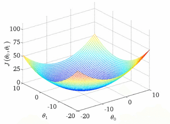
In reality, relevance is far messier. There’s no one magical optimum, but rather many local optimum depending on many other factors! Why? In other words, relevance looks far lumpier like in this graph:

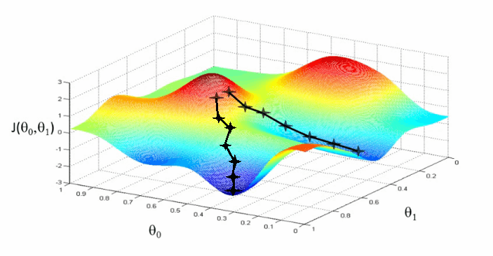
You can imagine these graphs (courtesy of Andrew NG’s ML class) as showing the ‘relevance error’ – how far are we from the grades we’re learning. The two theta variables map to say the title and overview relevance scores. In the first graph there’s a single optimum value that minimizes the “relevance error.” – an ideal set of boosts to apply to these two queries. The second is more realistic: lumpy, context-dependent minima. Sometimes a very high title boost value matters – othertimes a very low title boost!

Context and nuance matter!

Getting out of line!

That’s it for now. In future blog posts, I want to work on quantifying exactly where this model falls apart. What measures can we use to evaluate how good the model is? That will be a great stepping off point to examining other methods that can do a better job of capturing nuance.

I write these things so you’ll write to me! If you have any feedback, or if you need to teach me a thing or two, please get in touch and tell me how I’m wrong (I really want to learn from you!). Don’t hesitate to reach out if OpenSource Connections can help you with our relevancy services.

Did you know we also offer Learning to Rank training courses?

This blog post was created with Jupyter Notebook: View the source!