 Daniel Wrigley
Category: Ecommerce
Improving e-commerce search often starts with being able to actually know what’s going on in your online shop search, and much of this knowledge may be gathered by analyzing how your users interact with the site. We typically call these interactions “signals”. This blog post shows how to explore and visualize e-commerce search signal data to get actionable insights with examples using SQL and Apache Superset.
Introduction to the Data & Tools
To explore and visualize e-commerce search signal data, we need three things:
- a dataset
- a system to store the data in
- a tool that enables us to do the fun stuff, which is exploring and visualizing the data.
If you want to follow along here’s a repository that helps you set up everything you need: https://github.com/o19s/visualizing-signals
AI-Powered Search Dataset
For this introduction, I’m using the signals dataset from AI-Powered Search by Trey Grainger, Doug Turnbull and Max Irwin. This dataset records details about user search events as rows following this schema of columns:
type: Type of user interaction: [query, click, add-to-cart, purchase].query_id: Unique session ID. This is a unique identifier for the query session that is used to tie together after which queries clicks, add-to-carts or purchases happen.user_id: This is especially important to capture when preparing to deliver personalized search functionality in the future.target: The target can contain one of two things: For signals wheretype=queryit is the user query string, and for signals of other types, it is the identifier of the product the user interacted with.signal_time: Describes when the signal happened, e.g.2019-07-31T08:49:07.311600
Data Storage in PostgreSQL
Our data model is fairly simple and there are various options for how we can store our data. For this introduction, I chose PostgreSQL, as it is easy to run, reliable, widely used and it works out-of-the-box with our analytics and visualization tool, Apache Superset. The docker-compose.yml file in the above mentioned repository shows an exemplary setup including an initialization script that creates a table and copies the signal data into it, which is a matter of two SQL commands:
Create a table with a schema:
CREATE TABLE IF NOT EXISTS signals (
    id SERIAL PRIMARY KEY,
    query_id VARCHAR( 50 ) NOT NULL,
    user_id VARCHAR ( 25 ) NOT NULL,
    type VARCHAR ( 25 ) NOT NULL,
    target VARCHAR ( 255 ) NOT NULL,
    signal_time TIMESTAMP NOT NULL
);
Copy the data into the created table:
COPY signals(query_id, user_id, type, target, signal_time)
  FROM '/signals.csv'
  DELIMITER ','
  CSV HEADER;
That’s it! The data is loaded into the database.
Apache Superset for Visualization
With the data available in PostgreSQL, we can now use Apache Superset’s features to explore and visualize the data. Apache Superset is a tool for exploratory data analysis and it can connect to a huge variety of data stores including traditional SQL databases like PostgreSQL or MySQL, as well as NoSQL platforms like Solr or Elasticsearch and even cloud options like Google Big Query or Amazon Redshift, which are becoming increasingly popular.
Visualize e-commerce search signal data with a basic dashboard
Now that we have data stored in a database and a tool that can connect to the database to visualize the data, let’s create a dashboard to generate insights that we can use to tune our e-commerce search.
Connecting Apache Superset to PostgreSQL
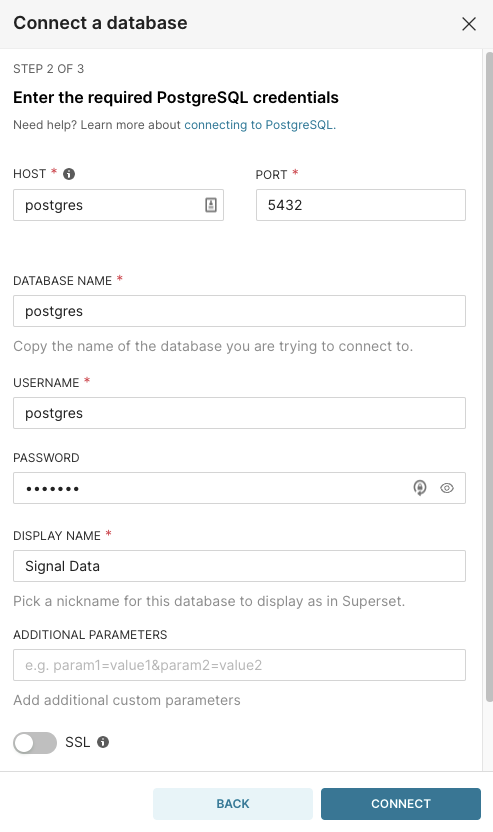
Apache Superset brings everything to the party that we need to connect to the database table that contains our e-commerce search signals. Once logged in, we can connect to a database by hitting the + DATABASE button in the databases section.

Following our example, we select PostgreSQL and specify the required credentials and settings:
- Host:
postgres - Port:
5432 - Database Name:
postgres - Username:
postgres - Password:
example - Display Name:
Signal Data
After connecting, Superset asks us if we want to create a dataset or query data in the SQL Lab. By choosing the second option, we can immediately start exploring the data.
Most Frequent Queries
By using the SQL Lab, we can query the data according to the question we want to have answered, and use the result in one of the various visualizations that are available. We’ll start with a basic question: “What are the most frequent queries that customers use to explore the product catalog?” Knowing the most popular queries, which we refer to as “head queries”, is very important because in making up the most traffic they are responsible for the biggest share of the overall revenue generated by e-commerce search.
The following SQL statement tells us the most frequent queries:
SELECT target AS target,
       count AS count
FROM
  (SELECT target,
          count(*)
   from signals
   WHERE type='query'
   GROUP BY target
   ORDER BY count DESC) AS virtual_table
LIMIT 1000;
The visualization type best suitable for this result is a table. Apache Superset gives us the option to create a chart based directly on this query. By selecting this option, we can save the result as a dataset and save the table as a chart by giving it a name.
Key Search Rates: Clickthrough, Add-to-Cart & Conversion
Search clickthrough rate (CTR) is a common KPI and in this case we are focusing on it. CTR is going to be the metric that answers the question “How often does a user click on a search result after they do a search?” We calculate this by dividing the number of clicks in distinct query sessions by the number of total query sessions and multiply the result by 100 to get the rate in percentage terms:
SELECT CAST(A.clicks AS FLOAT) / B.queries * 100 AS result
   FROM
     (SELECT count(distinct query_id) AS clicks
      FROM signals
      WHERE type='click') A,
     (SELECT count(DISTINCT query_id) AS queries
      FROM signals) B
From this SQL query, we get a floating point number. A number in a table may look unexciting but luckily other options exist for visualizing a number, especially a number that is a percentage. In Apache Superset we can use “Big Number” or “Gauge Chart”.
In our data setting, we have two additional types of rate signals that can happen after the click on a product in the hitlist: add-to-cart (ATC) and conversion rate (sometimes abbreviated as CVR). These answer these two questions:
- ATC: “How often does a user add a product to the cart after searching?“
- CVR: “How often does a user buy a product after searching?“
The calculations of these KPIs are very similar to the calculation of the CTR. We divide the number of add-to-cart events by the number of total query sessions and multiply the result by 100 and we do the same for the purchase events.
Retrieving the add-to-cart rate with SQL:
SELECT CAST(A.a2c AS FLOAT) / B.queries * 100 AS a2c_rate
   FROM
     (SELECT count(DISTINCT query_id) AS a2c
      FROM signals
      WHERE type='add-to-cart') A,
     (SELECT count(DISTINCT query_id) AS queries
      FROM signals) B
Retrieving the conversion rate with SQL:
SELECT CAST(A.purchases AS FLOAT) / B.queries * 100 AS cvr
   FROM
     (SELECT count(DISTINCT query_id) AS purchases
      FROM signals
      WHERE type='purchase') A,
     (SELECT count(DISTINCT query_id) AS queries
      FROM signals) B
Again, “Gauge Chart” and “Big Number” are both good options to visualize these kinds of rates.
Top & Low Performing Queries
Having global KPIs that allow us to do an aggregated assessment of how well search performs is great, but sometimes it is necessary to zoom in on the details at the query level. This view allows finding out what individual queries are top or low performing queries in a system, telling us which areas are ripe for improvement by our search team.
This view answers the question “What are our best and worst performing queries?”.
To get answers to these questions, we will be grouping the queries and calculating the query frequency, the number of purchases and the resulting conversion rate for each query. To see the best performing queries first, we sort by conversion rate in descending order and to see the worst performing queries first, we sort by conversion rate in ascending order.
Top performing queries:
SELECT query AS query,
       num_queries AS num_queries,
       num_purchases AS num_purchases,
       cvr AS cvr
FROM
  (SELECT query AS query,
          Y.num_queries,
          X.count AS num_purchases,
          Cast(X.count AS FLOAT) / Y.num_queries * 100 AS CVR
   FROM
     (SELECT query AS query,
             Count(*)
      FROM
        (SELECT A.target AS query,
                A.query_id
         FROM signals A,
              signals B
         WHERE A.query_id = B.query_id
           AND A.type = 'query'
           AND B.type = 'purchase'
           AND A.target <> B.target
         GROUP BY A.target,
                  A.query_id
         ORDER  BY query ASC) AS virtual_table GROUP  BY query
      ORDER  BY count DESC) X
   LEFT JOIN
     (SELECT target AS target,
             count AS num_queries
      FROM
        (SELECT target,
                Count(*)
         FROM signals
         WHERE type = 'query' GROUP  BY target
           ORDER  BY count DESC) AS virtual_table_queries) Y ON (Y.target = x.query)
   ORDER  BY CVR DESC,num_queries DESC) AS virtual_table
LIMIT 500;
Low performing queries:
SELECT query AS query,
       num_queries AS num_queries,
       num_purchases AS num_purchases,
       cvr AS cvr
FROM
  (SELECT query AS query,
          Y.num_queries,
          X.count AS num_purchases,
          ROUND(Cast(X.count AS DECIMAL(10, 2)) / Y.num_queries * 100.00, 2) AS CVR
   FROM
     (SELECT query AS query,
             Count(*)
      FROM
        (SELECT A.target AS query,
                A.query_id
         FROM signals A,
              signals B
         WHERE A.query_id = B.query_id
           AND A.type = 'query'
           AND B.type = 'purchase'
           AND A.target <> B.target
         GROUP BY A.target,
                  A.query_id
         ORDER  BY query ASC) AS virtual_table GROUP  BY query
      ORDER  BY count DESC) X
   LEFT JOIN
     (SELECT target AS target,
             count AS num_queries
      FROM
        (SELECT target,
                Count(*)
         FROM signals
         WHERE type = 'query' GROUP  BY target
           ORDER  BY count DESC) AS virtual_table_queries) Y ON (Y.target = x.query)
   ORDER  BY CVR ASC) AS virtual_table
LIMIT 500;
Putting the charts together in a Dashboard
Apache Superset lets us create a dashboard with all of the charts we created with the above SQL statements:
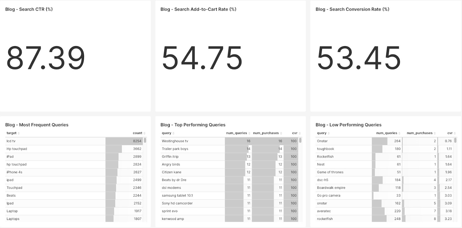
The top row describes the global view on the transactional KPIs CTR, add-to-cart rate and conversion rate – an overall view of how search is performing.
The bottom row shows metrics at the individual query level, allowing you to identify targets for improvement:
- Raw frequency
- Number of purchases
- Conversion rate
Actionable Insights
Now that we can visualise e-commerce search signal data using a dashboard with some charts in place, we can use it as a starting point for improving our search. The global numbers may be used as a measurement of the overall health of our system. Simply put, seeing drops in these rates over time can be seen as an indicator that something is going wrong, whereas increasing rates would tell us a story of successfully implemented search improvements.
Actionable insights can be generated out of the query level views on the metrics, and this is great, but this is really just a starting point. Looking at these queries and the associated numbers, we will start to have an idea about what kind of improvements we would like to get done, but it does not tell us how to make these changes.
However before we actually make changes, we need to measure the relevance of the search results our e-commerce search generates. To do that we need to be able to scientifically gather human ratings of the results on a defined quality scale, and calculate the overall effects and the extent of improvement or degradation of search result quality overall, using the law of averages to do “before and after” style comparisons. Quepid is a great tool for gathering these human ratings.
Many of the tools, steps and processes necessary to do so are described in our Meet Pete blog series covering the Chorus stack, which helps you take ownership of your overall search experience, and manage it so that you can more easily present your users the relevant search results they need. Chorus is a freely available open source reference implementation of a measurable and tunable e-commerce search platform.
If you need our help with measuring and tuning your e-commerce search contact us today!